The fastest Linux timestamps
26 Apr 2026Table of contents
Timing the timers
One of my pet projects at my last job was to introduce distributed tracing to a low-latency pipeline (think 1–10 microseconds per stage) using OpenTelemetry. As part of this effort I spent a considerable amount of time designing, implementing, and optimising our own C++ tracing client library, as the official one has too much overhead. My goal was for the latency impact per component to stay under 5% so both developers and users would feel comfortable leaving traces always on in production; this translated to a budget of about 50–100 ns (a few hundred clock cycles) per span.
As you might imagine, at this scale you must carefully consider every aspect of the design and implementation, from ID generation to serialisation. One of these not-so-small details is how to timestamp spans. OTLP uses two time fields, one each for the start and end of the span as measured by the local wall clock. Although the end time is an absolute timestamp, it’s expected that it will always be later than the start time, as its primary purpose is to measure the span duration. The official client handles this roughly as:
Span::Span(/* ... */)
{
    // ...
    start_time_ = std::chrono::system_clock::now();
    start_steady_time_ = std::chrono::steady_clock::now();
    // ...
}

void Span::End(/* ... */)
{
    // ...
    auto end_steady_time = std::chrono::steady_clock::now();
    auto duration = end_steady_time - start_steady_time_;
    end_time_ = start_time_ + duration;
    // ...
}
It takes the start time from the real-time clock and uses two timestamps from the monotonic clock to calculate a nonnegative span duration without interference from discontinuous system clock adjustments. The end time is a synthetic timestamp obtained by adding the duration to the start time, rather than directly from any clock.
Does querying the system clocks three times per span have any significant performance impact? If
you’re at all familiar with Linux internals, you might expect the answer to be no: after all, in
practically any application using the C library the clock_gettime() syscall (indirectly called by
the now() functions) will be routed through vDSO to avoid context-switching into the kernel.
Let’s do a quick benchmark to confirm:
void BM_NaiveBackToBack(benchmark::State& state)
{
    for (auto _ : state) {
        auto ts = std::chrono::system_clock::now();
        auto start = std::chrono::steady_clock::now();
        auto duration = std::chrono::steady_clock::now() - start;

        benchmark::DoNotOptimize(ts + duration);
    }
}
On my laptop1 (see the appendix for details on the setup) this yields iteration times between 46 and 49 ns—almost our entire time budget for a span, spent just on timestamping! Clearly this will not suffice.2
If we’re to meet our latency constraints, we’ll need to understand how Linux clocks work under the hood and find out how much weight we can shed. We’ll see what the x86 timestamp counter is and how it works, do a deep dive into the implementation of vDSO, and use our newly acquired knowledge to chop over 50% of the timing overhead from our initial attempt. All the benchmarking code is available. If you’re already familiar with the TSC and vDSO internals feel free to skip to the good stuff.
The TSC
Almost anyone who has written microarchitecture benchmarks or otherwise needed fast and accurate timestamps on x86 platforms is well acquainted with the CPU’s timestamp counter, or TSC. Quoting from Intel’s System Programming Guide:
The time-stamp counter […] is a 64-bit counter that is set to 0 following a RESET of the processor. Following a RESET, the counter increments even when the processor is halted by the HLT instruction or the external STPCLK# pin.
The time stamp counter in newer processors may support an enhancement, referred to as invariant TSC. […] The invariant TSC will run at a constant rate in all ACPI P-, C-. and T-states. This is the architectural behavior moving forward. On processors with invariant TSC support, the OS may use the TSC for wall clock timer services (instead of ACPI or HPET timers). TSC reads are much more efficient and do not incur the overhead associated with a ring transition or access to a platform resource.
(By “newer processors” in the second paragraph we should understand any relatively modern CPU,
really. You can confirm whether this is the case on your machine by looking for the constant_tsc
and nonstop_tsc flags in /proc/cpuinfo.)
An invariant TSC behaves exactly as you would expect from a clock: it’s fully synchronised across cores (so it doesn’t matter from which one you read it), runs at a constant rate independent of frequency scaling3, and doesn’t stop even when the system is idle or suspended. It’s still, of course, subject to frequency deviations like any other clock, which is one reason why NTP or PTP synchronisation is important.
Although, as the manual suggests, TSC reads are in fact much more efficient than the alternatives,
they’re not free. The cost of reading the TSC is twofold: the instruction itself is slow (rdtsc
has a reciprocal throughput of 25 core clock
cycles on Skylake) and the instruction
stream must be serialised first, either through an explicit lfence or by using rdtscp4
(32 cycles), so that all preceding instructions execute before we read the counter; otherwise we can
easily introduce errors of 10-30%, depending on the workload.
When syscalls aren’t
I won’t spend much time explaining what the vDSO itself is, as the man
page does a pretty good job. The long and short
of it is that when a user-space process invokes certain system calls through the C library (most
notably, clock_gettime()), the library directs that call to a small shared library mapped into the
process (the vDSO), which avoids the overhead of switching into ring 0 by reading the required
information from a memory region shared with the kernel, called the vvar or data page.
The data page is
placed four
pages before the vDSO mapping itself and
contains two vdso_data
structures (one for the high-resolution clock, subject to frequency adjustments, and one for the raw
clock) at offset
128. We can find the
vDSO code to read from these structures in
lib/vdso/gettimeofday.c.
We’re particularly interested in the do_hres()
function, which is used
for all calls to high-resolution clocks such as CLOCK_REALTIME and CLOCK_MONOTONIC
(corresponding to system_clock and steady_clock, respectively). Here’s a simplified version of
the function assuming an x86 target without time namespaces and an invariant TSC:
static int
do_hres(const struct vdso_data *vd, clockid_t clk, struct __kernel_timespec *ts)
{
    const struct vdso_timestamp *vdso_ts = &vd->basetime[clk];
    u64 cycles, last, sec, ns;
    u32 seq;

    do {
        seq = vdso_read_begin(vd);
        cycles = __arch_get_hw_counter(vd->clock_mode, vd);
        ns = vdso_ts->nsec;
        last = vd->cycle_last;
        ns += (cycles - last) * vd->mult;
        ns = ns >> vd->shift;
        sec = vdso_ts->sec;
    } while (unlikely(vdso_read_retry(vd, seq)));

    ts->tv_sec = sec + __iter_div_u64_rem(ns, NSEC_PER_SEC, &ns);
    ts->tv_nsec = ns;

    return 0;
}
The way it works is as follows: on every kernel tick, the CPU responsible for updating the timers does a bunch of math to advance the system clock and updates the data page with the resulting values. This is the kernel’s best estimate of the current time for each clock, along with the current cycle count of the underlying clock source (on x86, of course, the TSC) and a multiplier/shift pair to efficiently convert cycles into nanoseconds (essentially a fixed-point representation of the estimated clock period). The whole structure is protected by a seqlock: the kernel increments the sequence number before and after each update so readers can recognise when an update is in progress (the sequence number is odd) or when it occurred during the read (the sequence number changes).
Back in userspace, all do_hres() needs to do is load the values from the page, get the current
cycle count from the TSC (through __arch_get_hw_counter(), which uses lfence+rdtsc or rdtscp
if available), convert the difference to a nanosecond offset, and finally fold the excess amount
into the seconds value.
Faster monotonic clocks
Because all the heavy lifting is done in the kernel, calls to clock_gettime() through vDSO are
quite efficient for most purposes. But there is still some extraneous work slowing down our use
case:
-
Even though the only difference between the wall clock and the monotonic clock is the base time, we need to do two initial calls to get both timestamps, duplicating the critical region, several loads, the conversion from cycles to nanoseconds, the division into seconds, and above all the expensive TSC read. (Reading the TSC twice also means we use two slightly different timestamps for the start of the span.)
-
Because we only use the monotonic clock to measure a time interval, we could skip the calculation of timestamps and convert only the cycle difference to nanoseconds using the multiplier and shift values:
delta = ((cycles_end - cycles_start) * mult) >> shift. -
Because OpenTelemetry timestamps are in nanoseconds since the epoch, we don’t need to normalise the seconds field or even calculate it at all. Although this does not use an actual division instruction, it still carries a cost.
Let’s see if we can reach a solution that addresses all of these points. To start, we’ll refactor our initial timing logic into its own class so we can more easily benchmark different approaches:
class NaiveTimer
{
public:
    using duration = std::chrono::steady_clock::duration;
    using time_point = std::chrono::system_clock::time_point;

    time_point start() noexcept
    {
        const auto ts = std::chrono::system_clock::now();
        start_ = std::chrono::steady_clock::now();
        return ts;
    }

    duration elapsed() const noexcept
    { return std::chrono::steady_clock::now() - start_; }

private:
    std::chrono::steady_clock::time_point start_;
};
As I mentioned earlier, the standard way to measure time intervals with low overhead on x86 is by directly reading the TSC. We can replace our calls to the monotonic clock as follows5:
static inline __attribute__((always_inline)) uint64_t rdtsc()
{
    uint32_t id;
    return __rdtscp(&id);
}

template <typename Estimate>
class TscTimer
{
public:
    using duration = std::chrono::duration<int64_t, std::nano>;
    using time_point = std::chrono::system_clock::time_point;

    time_point start() noexcept
    {
        const auto ts = std::chrono::system_clock::now();
        start_ = __rdtsc();
        return ts;
    }

    duration elapsed() const noexcept
    {
        const auto end = rdtsc();
        return duration{Estimate::ns_from_cycles(end - start_)};
    }

private:
    uint64_t start_;
};
I encapsulated the conversion from cycles to nanoseconds in a separate template parameter so we can measure the overhead of different methods. There are essentially two ways to do this conversion: dividing by the frequency or multiplying by the period, which should be significantly faster. I will skip the details of the estimation itself, as they’re not relevant to our purposes (but see the implementation).
An interesting thing about TscTimer is that we don’t need explicit serialisation in start()
because, as we have seen, clock_gettime() itself already serialises the instruction stream; we
only need to do it again if we really want to exclude the instructions in-between from our
measurement.
How much of an improvement do we get with our new timers?
| Timer | Median time (ns) | Gain |
|---|---|---|
| Naive | 47.2 | — |
TscTimer with frequency estimate |
33.8 | 28% |
TscTimer with period estimate |
28.3 | 40% |
Not bad! We have addressed most of points 1 and 2 without much effort for a substantial gain. As expected, using a multiplication for the conversion to nanoseconds instead of an integer division also helps quite a bit. But we’re still reading the TSC twice at the beginning and unnecessarily converting to and from a split seconds/nanoseconds representation. Can we go further?
Making our own vDSO
We know that the vDSO doesn’t have any special, privileged access to the kernel; ultimately, it simply provides a convenient interface to read the data on the vvar page. There’s nothing stopping us from implementing our own logic to do this too, tailored to our own needs; all we need is the layout of the page, which we already have, and its address. A closer reading of the man page tells us:
The base address of the vDSO (if one exists) is passed by the kernel to each program in the initial auxiliary vector (see
getauxval(3)), via theAT_SYSINFO_EHDRtag.
Since we know the vvar page is located four pages before the vDSO mapping, we can easily get a pointer to the clock data:
static constexpr size_t VVAR_OFFSET = 4;
static constexpr size_t VDSO_DATA_OFFSET = 128;

static const vdso_data* get_vdso_data()
{
    auto page_sz = sysconf(_SC_PAGESIZE);
    auto vdso = getauxval(AT_SYSINFO_EHDR);
    auto vvar = vdso - VVAR_OFFSET * page_sz;
    return reinterpret_cast<const vdso_data*>(vvar + VDSO_DATA_OFFSET);
}
Now we just draw the rest of the owl:
class VdsoTimer
{
public:
    using duration = std::chrono::duration<int64_t, std::nano>;
    using time_point = std::chrono::time_point<std::chrono::system_clock, duration>;

    time_point start() noexcept { return time_point{read_clock(data)}; }

    duration elapsed() const noexcept
    {
        auto cycles = rdtsc();
        return duration{((cycles - start_) * mult_) >> shift_};
    }

private:
    static constexpr uint64_t NS_PER_SEC = 1'000'000'000UL;

    duration read_clock(const vdso_data* vd)
    {
        auto rt = &vd->basetime[CLOCK_REALTIME];
        uint64_t cycles, last, sec, ns;
        uint32_t seq, mult, shift;

        auto vseq = std::atomic_ref{vd->seq};

        do {
            while ((seq = vseq.load(std::memory_order_acquire)) & 1)
                _mm_pause();

            cycles = rdtsc();
            sec = rt->sec;
            ns = rt->nsec;
            last = vd->cycle_last;
            mult = vd->mult;
            shift = vd->shift;
        } while (seq != vseq.load(std::memory_order_acquire));

        ns += (cycles - last) * mult;
        ns >>= shift;

        start_ = cycles;
        mult_ = mult;
        shift_ = shift;

        return duration{sec * NS_PER_SEC + ns};
    }

    static inline const vdso_data* const data = get_vdso_data();

    uint64_t start_;
    uint32_t mult_;
    uint32_t shift_;
};
There are a few implementation choices here that require some elaboration:
-
Using C++ atomics to handle the seqlock gives us the correct semantics for free without having to worry about the details of atomicity, memory ordering, or compiler barriers, even on other architectures like ARM with weaker guarantees.
-
We use a
pauseinstruction in the busy-wait loop (just as the kernel does) as a hint to the processor to avoid memory order violations on exit that might cause it to flush the pipeline. On some architectures, such as Skylake, this instruction can be exceedingly slow (~140 cycles) and might not be worth it. -
Reading the TSC inside the loop, as in the original vDSO implementation, improves median performance by not waiting for the loads from the data page to finish. This does mean that our measurement includes the cycles used by these instructions, but since any potential cache misses must already have occurred when loading
seqthe difference will be minimal. Conversely, if we want to make sure to include the full timer overhead we can move the read before the loop. -
Instead of loading the multiplier and shift from the data page at the end of the interval, we cache them in the timer itself at the cost of an extra 8 bytes, avoiding entering the critical region again and the attendant possibility of a cache miss after an update.6
- I chose to let the compiler inline the start/stop methods in the benchmarks since that’s how they
would be used in a tracing library. In other applications you may choose to
no_inlinethe start method to avoid growing the code size and taking up space in the branch prediction unit, at the cost of a few extra cycles (elapsed()is small enough and has no branches so there’s no gain doing that).
Note that, unlike with TscTimer, VdsoTimer uses the kernel’s current best estimate of the TSC
frequency to calculate the time difference. This way, not only do we avoid having to make our own
estimate but we also take advantage of the kernel’s clock synchronisation (e.g. through NTP), making
our measurements more precise.
Time to see what our efforts have gained us:
| Timer | Median time (ns) | Gain |
|---|---|---|
| Naive | 47.2 | — |
TscTimer with period estimate |
28.3 | 40% |
VdsoTimer |
20.5 | 57% |
We managed to cut over half of our initial timing overhead! As small as these differences might be in absolute terms, cumulatively over the whole library they’re significant enough that we can go from “we turn tracing on for debugging” to “tracing is on by default”.
We can confirm that we’re not chasing ghosts by timing a simulated computational load (calculating a Collatz trajectory) calibrated to take 1 μs. For completeness, I also added a non-monotonic timer which uses only the wall clock to measure the interval, to show how discarding the monotonicity requirement by itself is not enough to get the same results:
| Benchmark | Median time (ns) | Overhead |
|---|---|---|
| Baseline | 1000 | — |
| Naive timer | 1043 | 4.3% |
| Non-monotonic timer | 1027 | 2.7% |
TscTimer with period estimate |
1027 | 2.7% |
VdsoTimer |
1020 | 2.0% |
The overhead is largely in line with the back-to-back benchmarks; there’s not a lot of opportunity for ILP or reordering to hide the timing latency due to the need to serialise execution.
Measuring tails
At this point, the five of you who care enough about performance to be here might be screeching incoherently about tail latencies and 99th percentiles. Fear not, gentle reader, I have not forsaken you.
The one problem all of the approaches we have seen so far have in common is what happens when the kernel updates the data page, which as we know happens on every tick. An update slows down the timer in two ways. The most obvious one is that the caller might have to spin waiting for the update to finish; the other is that we have L1 and L2 cache misses on the vDSO data7: one if the update already happened (all the data is cache-aligned and fits in a single line), and two or more if it’s ongoing or starts while we load the data, bouncing the cache line between cores.
To capture these events we need to write our own benchmark that averages the duration of a small number of calls, repeated many times over a relatively long period (tens of milliseconds). To distinguish the three cases I have just described we’ll use the CPU performance counters to measure the number of retired instructions and L1 cache misses, as well as the elapsed time measured from the TSC. This is what we expect to see:
| # | Update since last call | Cache misses | Retired instructions | Duration |
|---|---|---|---|---|
| 1 | No | 0 | Baseline | ~Constant |
| 2 | Yes, complete | 1 | Baseline | Slower |
| 3 | Starting or ongoing | 2+ | Higher | Slowest |
We’ll read each counter before and after each run of 100 paired, back-to-back start()/elapsed()
calls for each timer, so we can sufficiently amortise the measurement overhead while ensuring
there’s at most one update per run. I won’t go over the
implementation here, but let’s
analyse the results. Here’s the average duration per run per timer over the whole benchmark8:
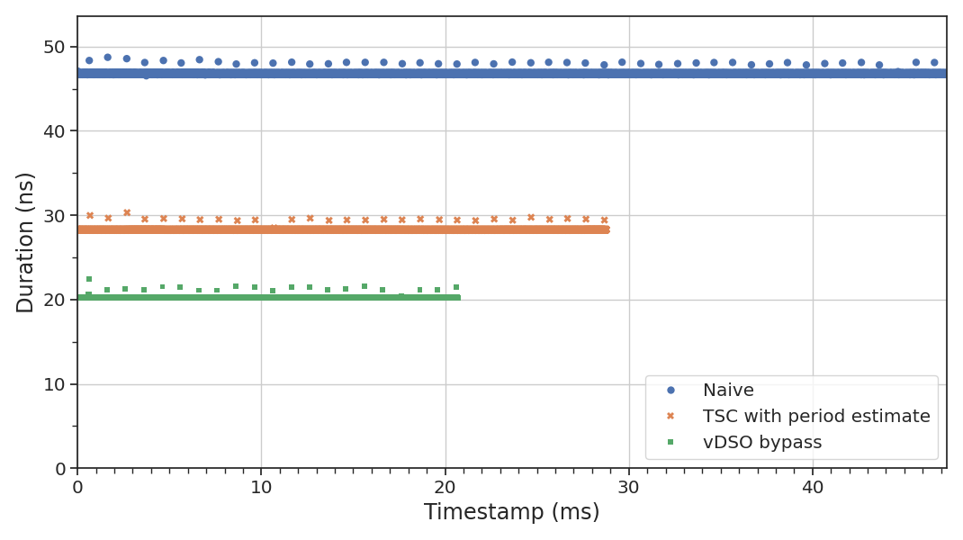
The dots above the baseline for each timer, at precisely spaced 1 ms intervals (my kernel is
compiled with HZ = 1000), show the effect of updates to the data page on our runtime. Since the
y-axis is averaged over 100 calls, and we have at most one update per run, the actual tail latency
impact is a hundred times higher than it appears on the graph:
Even with our vDSO bypass timer, we can still have tail latencies in excess of 200 ns above the median—4x higher than our total time budget for a span. Not ideal!
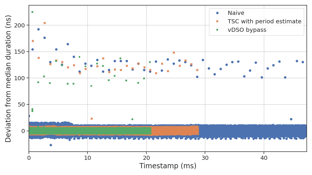
We can also look at the total L1 cache misses versus the number of additional retired instructions for the vDSO bypass to confirm our earlier hypothesis:
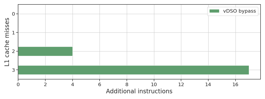
The cases with one cache miss correspond to scenario 2 in the table above (a complete update happened
between the call to elapsed() and the next start()), and as expected show no matching increase
in retired instructions. You can also see these represented in the duration graph as the three runs
with deviations from the median around 20 ns. The other cases (two and three misses) correspond to
scenario 3, where we need to spin waiting for the update to finish.
Stable timers
Although we have significantly reduced the median latency impact of our timer, we’re still left with
undesirable tails significantly above our target. The problem is that every call to start() runs
the risk of either catching the kernel mid-update or otherwise incurring an L2 cache miss due to
a previous update.
What if we didn’t have to read from the data page on every call? Stable systems rarely or never
have discontinuous clock adjustments, and the frequency adjustments are gradual enough that it won’t
matter if we miss a few—assuming we even care to track them at all. Instead, we can cache the
required data ourselves9 and refresh it at some acceptable frequency (below or equal to
HZ) as part of our main event loop whenever we know we have enough cycles to spare. This also
allows us to pre-compute the conversion from seconds to nanoseconds, saving us a load,
a multiplication, and an addition:10
class VdsoCacheTimer
{
public:
    static void refresh() noexcept { cache = read(vd); }

    time_point start() noexcept { return time_point{read_clock(data)}; }

    duration elapsed() const noexcept
    {
        auto cycles = rdtsc();
        return duration{((cycles - start_) * cache.mult) >> cache.shift};
    }

private:
    struct VdsoCache
    {
        uint64_t last, ns;
        uint32_t mult, shift;
    };

    // ...

    duration read_clock() noexcept
    {
        auto cycles = rdtsc();
        start_ = cycles;
        auto d = ((cycles - cache.last) * cache.mult) >> cache.shift;
        return duration{cache.ns + d};
    }

    static inline const vdso_data* const vd = get_vdso_data();
    static inline VdsoCache cache = read(vd);

    uint64_t start_;
};
But now that we have cached the current time for the vDSO bypass, can’t we just do the same for
TscTimer? Indeed we can, giving us our final line-up:
| Timer | Median time (ns) | Gain |
|---|---|---|
| Naive | 47.2 | — |
TscTimer with period estimate |
28.3 | 40% |
TscCacheTimer |
19.6 | 58% |
VdsoTimer |
20.5 | 57% |
VdsoCacheTimer |
20.0 | 58% |
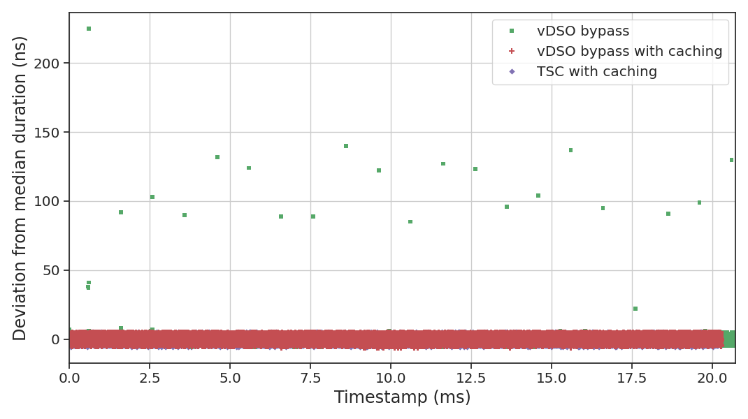
Both implementations completely avoid the latency tails that plagued other approaches, as expected.
The cached TSC timer has a tiny performance advantage over VdsoCacheTimer (around 0.1 cycles per
iteration) due to the use of a hardcoded shift, while VdsoCacheTimer has a slight edge on accuracy
since it tracks the TSC frequency measured by the kernel and only reads the TSC once on refresh.
Conclusion
We have implemented two efficient timers with highly predictable performance (no tails and tight
clustering around the median), but there is an obvious downside to bypassing the vDSO: whenever the
layout of the data page changes, as in Linux 6.15, we have to update our implementation accordingly.
Therefore, for almost all applications that need to worry about this in the first place
TscCacheTimer will be a better choice, as long as the small loss of precision is not an issue.
What’s more important to understand, and more generally applicable, is that typical benchmarks only ever present part of the picture; if you need highly-predictable latency, you cannot rely exclusively on statistical averages to characterise your components. Just as relevant is understanding what lies beneath the abstractions we rely on in order to make informed guesses as to what might affect their performance and under what circumstances, so we’re not stuck mindlessly playing whack-a-mole with cache miss or branch misprediction counters.
Appendix: Methodology
All benchmarks were compiled with clang-20 with -O2 -march=x86-64-v3 -fno-unroll-loops flags and
executed on Ubuntu 24.04 with Linux kernel 6.8.0, on an Intel Core i7-8565U processor with four
cores in a single socket. Core 3 was isolated at boot using isolcpus=3 nohz_full=3 rcu_nocbs=3
kernel command-line arguments and the benchmark processes pinned to it. Hyper-threading was
disabled and the intel_pstate driver put in passive mode. All cores were configured to use the
performance governor with a fixed 4.1 GHz frequency (the highest operating frequency sustained by
the CPU on all four cores).
CPU details
Architecture:                x86_64
  CPU op-mode(s):            32-bit, 64-bit
  Address sizes:             39 bits physical, 48 bits virtual
  Byte Order:                Little Endian
CPU(s):                      8
  On-line CPU(s) list:       0-3
  Off-line CPU(s) list:      4-7
Vendor ID:                   GenuineIntel
  Model name:                Intel(R) Core(TM) i7-8565U CPU @ 1.80GHz
    CPU family:              6
    Model:                   142
    Thread(s) per core:      1
    Core(s) per socket:      4
    Socket(s):               1
    Stepping:                12
    CPU(s) scaling MHz:      89%
    CPU max MHz:             4600,0000
    CPU min MHz:             0,0000
    BogoMIPS:                3999,93
    Flags:                   fpu vme de pse tsc msr pae mce cx8 apic sep mtrr pge mca cmov pat pse36 clflush dts acpi mmx fxsr sse sse2 ss ht tm pbe syscall nx pdpe1gb rdtscp lm constant_tsc art arch_perfmon
                             pebs bts rep_good nopl xtopology nonstop_tsc cpuid aperfmperf pni pclmulqdq dtes64 monitor ds_cpl vmx est tm2 ssse3 sdbg fma cx16 xtpr pdcm pcid sse4_1 sse4_2 x2apic movbe popcnt
                             tsc_deadline_timer aes xsave avx f16c rdrand lahf_lm abm 3dnowprefetch cpuid_fault epb ssbd ibrs ibpb stibp ibrs_enhanced tpr_shadow flexpriority ept vpid ept_ad fsgsbase tsc_adju
                             st bmi1 avx2 smep bmi2 erms invpcid mpx rdseed adx smap clflushopt intel_pt xsaveopt xsavec xgetbv1 xsaves dtherm ida arat pln pts hwp hwp_notify hwp_act_window hwp_epp vnmi md_cl
                             ear flush_l1d arch_capabilities ibpb_exit_to_user
Virtualisation features:
  Virtualisation:            VT-x
Caches (sum of all):
  L1d:                       128 KiB (4 instances)
  L1i:                       128 KiB (4 instances)
  L2:                        1 MiB (4 instances)
  L3:                        8 MiB (1 instance)
NUMA:
  NUMA node(s):              1
  NUMA node0 CPU(s):         0-3
Vulnerabilities:
  Gather data sampling:      Mitigation; Microcode
  Indirect target selection: Mitigation; Aligned branch/return thunks
  Itlb multihit:             KVM: Mitigation: VMX disabled
  L1tf:                      Not affected
  Mds:                       Not affected
  Meltdown:                  Not affected
  Mmio stale data:           Mitigation; Clear CPU buffers; SMT disabled
  Reg file data sampling:    Not affected
  Retbleed:                  Mitigation; Enhanced IBRS
  Spec rstack overflow:      Not affected
  Spec store bypass:         Mitigation; Speculative Store Bypass disabled via prctl
  Spectre v1:                Mitigation; usercopy/swapgs barriers and __user pointer sanitization
  Spectre v2:                Mitigation; Enhanced / Automatic IBRS; IBPB conditional; PBRSB-eIBRS SW sequence; BHI SW loop, KVM SW loop
  Srbds:                     Mitigation; Microcode
  Tsa:                       Not affected
  Tsx async abort:           Not affected
  Vmscape:                   Mitigation; IBPB before exit to userspace
Benchmarks were compiled and executed separately for each timer. The table measurements for back-to-back calls are the medians of 100 thousand runs, each averaged over 100 iterations; the measurements for the simulated task, as well as each graph, represent 10 thousand runs.
-
A laptop with a mobile processor is, of course, a far cry from the overpowered CPUs used in datacentres, so the actual numbers are not directly comparable. However, for our purposes the relative differences between benchmarks are what matters most, and those do not change significantly. ↩
-
One of the perils of microbenchmarking is that we can be led down a rabbit hole of optimisations that look good in isolation but have no or negative impact in production. We might wonder if this benchmark is entirely fair to “naive” timestamping; maybe when integrated in our codebase most of the impact would be absorbed by the execution pipeline or the reordering buffer. We will see later why this is not the case. ↩
-
It seems to be a popular misconception that the TSC frequency is the same as the base CPU clock frequency, but this is not the case. Until recently, in fact, the most reliable way to determine the TSC frequency was to directly estimate it using a separate, reliable timer (such as HPET). For example, on my laptop:
$ sudo dmesg | grep MHz [ 0.000000] tsc: Detected 2000.000 MHz processor [ 0.000000] tsc: Detected 1999.968 MHz TSC [ 1.398488] tsc: Refined TSC clocksource calibration: 1991.999 MHz -
This is not entirely correct, as per the manual
rdtscpis not a serialising instruction. It does wait until all previous instructions have executed, just likelfence, but the latter also explicitly prevents all subsequent instructions from executing (even speculatively) until it completes. In practice, unless you’re measuring microarchitectural features of the processor, they amount to the same result. ↩ -
I’m using x86 intrinsics here (from
x86intrin.h) rather than inline Assembly for simplicity of exposition; the generated code, however, is identical. ↩ -
This may produce slightly different measured values than our initial approach in case the multiplier is updated during the timed interval (the shift is never updated after initialisation), but the difference should be irrelevant in practice. We could also just load the multiplier from the page without locking, since 64-bit stores and loads are guaranteed to be atomic, but this can still trigger an L2 cache miss. ↩
-
This assumes that the scheduler does not run on the same core where we run the timer, as is the case with any low-latency workload running on isolated cores. If that’s not true the context switch dominates the total latency anyway and you have bigger problems to fix. ↩
-
The total duration of the benchmark changes because we have a fixed number of runs for each timer. ↩
-
We can make the cache thread-local for multi-threaded applications, although to maintain performance we need to store a pointer to the current thread’s cache in each timer. ↩
-
The code clang-20 generates for this implementation is sub-optimal due to some questionable ordering choices that don’t fully take advantage of ILP, as well as the use of RIP-relative addressing to access the data (which increases the average instruction length, saturating the fetch unit). The benchmark numbers below for both
VdsoCacheTimerandTscCacheTimerare for a fine-tuned implementation that uses general-purpose registers more aggressively. ↩